Computational Modeling of Stents in Arteries

 

The finite element method has become the most widely used computational technique in solving the governing equations (conservation of linear momentum) for solids.  However, there exist many other computational methods besides the Galerkin finite element method.  These include the subdomain method, the finite volume method, Field/Boundary Element Method, and the meshless local Petrov-Galerkin method.  Many of the previously mentioned computational methods are based on the weighted residuals method (weak form) in which the weighted average of the error of the differential equation is set to zero over the domain under study.  All these methods require the use of trial functions (to approximate the solution) as well as test functions (to form the weight function).  These functions must satisfy certain continuity requirements, such as C⁰, C¹, C², etc.  For instance, if in the differential equation, the n^th derivative of the dependent variable is present, then the trial solution’s (n-1)^th derivative must be continuous in order for it to make sense mathematically.  In other words, the trial solution must be C^n-1 continuous [13].  

As mentioned earlier, many computational methods are based on the weak form approach.  For the conservation of linear momentum (please see Solid Mechanics), the general weak form is

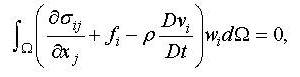
where Ω is the domain and w_i is the test (weight) function.  If the divergence theorem is used, then this equation can be expressed as

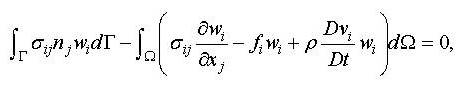
where Γ is the boundary and n_i is the outward normal vector to the boundary [13].  The finite element method is based on the symmetric weak form approach.  Before these equations can be solved, the constitutive equations of the different materials and the boundary conditions are needed.  It is important to note that because of the constitutive equation for a given material, the Cauchy stresses are actually functions of the displacement u_i.  As described in the section Solid Mechanics, the second Piola-Kirchhoff stresses S_ij and Cauchy stresses σ_ij can be expressed as

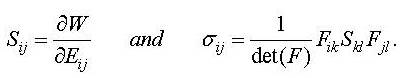
where E_ij is the Green strain tensor and F_ij is the deformation gradient tensor [7].  Thus, the constitutive equation for a given material can be expressed as

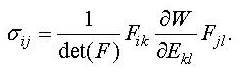
where W is the strain energy function for a specific material.  Note that the components of F_ij and E_ij are functions of the displacement vector u_i.  Furthermore, the boundary conditions specified in terms of some displacement or traction distribution on certain boundaries:

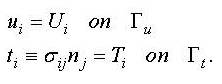
Then the weak form can be solved by assuming some trial functions ui for the displacement and by assuming some test functions w_i.  Global functions can be used, in which u_i and w_i can be polynomial functions over the entire global domain of the problem.  However, this usually does not work well, especially for global domains that have arbitrary shapes.  Instead, it is easier divide up the entire domain into very small elements (the finite elements) and use local functions for each of these subdomains.  Then the weak form becomes

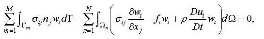
where M is the number of sub-boundaries and N is the number of subdomains.  The process of discretizing the domain into the finite elements is known as mesh generation [5].  In each of these finite elements, element nodal coordinates will be used as well as local basis functions (or element basis functions).  In other words, the trial and test functions used in each subdomain are different.  After assuming some form for these trial and test functions, the task is to solve for the undetermined coefficients in each of these local functions.  This involves the assembly of a large system of algebraic equations and then solving for all the unknowns (undetermined coefficients) in the system [13].  There are many commercial software that can implement the finite element method for the user; these include ABAQUS, ANSYS, and COMSOL.